Study area
The study area covers the Glenelg Hopkins (GH) region in the western part of Victoria State in Australia (Fig. 1). The region encompasses 2.67 million hectares that extend west from Ballarat to the South Australian border and south to the coast. It comprises 12% of the total area of Victoria45. The north is dominated by the Grampians, the Dundas and Merino Table Lands, and the West Victorian Uplands, with the flatter Volcanic Plains characterizing the south. The slope is prominent in the Grampian region, ranging from 100 down to 0% in the Volcanic Plains, with an average slope of 3.48% in the rest of the territory. Maps were produced using ArcMap 10.4.1 https://desktop.arcgis.com/en/arcmap/10.4/get-started/setup/arcgis-desktop-quick-start-guide.htm
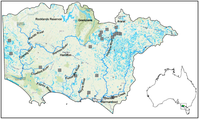
Glenelg Hopkins Catchment Management Authority in Victoria, Australia. Grey squares are monitoring bores for groundwater pollution.
Warrnambool and Casterton are the two major towns in the GH region. The mean annual maximum temperature in Warrnambool and Casterton is 19.2 °C and 20.1 °C, with a high of 38.3 °C and 38.5 °C in 2017, respectively. The mean annual minimum temperature in Warrnambool and Casterton is 8.9 °C and 8.4 °C, and the lowest in 2017 was −1.0 °C and −3.0 °C, respectively (BoM accessed March 2018). There are two distinct climates: Csb is temperate with dry and warm summers, and Cfb is temperate with dry winters and warm summers46.
The hydrological subregions are the Hopkins River Basin (East), which includes the Hopkins and the Merry rivers; the Portland Coastal (Southcentral), which includes the Moyne, Eumeralla, Fitzroy and Surry rivers; and the Glenelg River Basin (Northcentral and West), which includes the tributaries of the Glenelg River. The largest water body in the basin is the Rocklands Reservoir45.
Different soil lithologies are present in the region, with the most abundant lithologies including basalts, sedimentary, duricrust, and aeolian, followed by alluvium, limestone, alluvial, granite, colluvial, lacustrine/aeolian, and volcanic. The least abundant soils are fluvial, aeolian and lagoonal45. The hydrogeological features of the study area can be seen in Fig. 2.
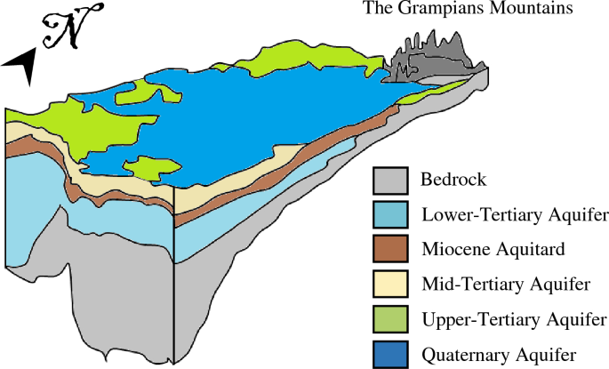
Cross-section of the hydrogeological units in the Glenelg Hopkins region.
Methods
We developed a novel method comprising five steps: (1) Data preparation. (2) Calculation of the Pesticide DRASTICL vulnerability index (IDL) using dynamic factors (D and R) and static hydrogeological factors (A, S, T, I, C, and L). (3) Independent computation of the correspondence analysis (CA) for both dynamic and static factor groups. (4) Upscaling the resulting eigenvalues to the Pesticide DRASTICL weight scale (1 to 5). (5) Recalculation of the seasonal IDL using the calculated weights from step 4.
The sources of data used for Pesticide DRASTICL factors are summarized in Table 1. Both dynamic factors were estimated with models: for D, we used HydroSight39, and for R, we used data resulting from the groundwater transient model for the Glenelg Hopkins Catchment Management Authority (CMA). The transient model included a three-stage approach: pre-development—1985, calibration—1985 to 1994, verification—1995 to 1999 and post-development—1995.
Computation of the Pesticide DRASTICL vulnerability index (IDL)
The Pesticide DRASTICL index is calculated summing the weight of all factor weight values times their corresponding rating value as presented below:
$$ I_{PDL} = \mathop \sum \limits_{1}^{i} r_{i} *w_{i} $$
(1)
where IPDL = Pesticide DRASTICL index (dimensionless).w = factor weight (dimensionless)r = rating for the corresponding range (dimensionless)
The modified weighting factor values are shown in Table 2. Weights represent how important each factor is when compared to others and range from 1 to 5, with 5 being the most significant factor and 1 the least significant factor30. Each factor was reclassified by assigning the corresponding rating value and converted to raster format using ArcMap10.4.1. Each factor layer was portrayed in a grid of 50 m × 50 m using a georeferenced GDA 1994 Lambert Conformal Conic projection. Ranges represent the significant media type that contributes to the pollution potential, and such values change spatially and within their own scale30. Every range is evaluated against each other to calculate the relative significance in relation to pollution potential30. In DRASTIC methods, the factor range of relative significance is evaluated on a scale of 1 (least significant) to 10 (most significant), except for the net recharge factor, which has a scale of 1 to 9.
Rating values were established using an ordinal scale; however, assigning range values from 1 to 10 to differentiate the relative importance between ranges has been found to be contrary to what can be truly comprehended, as the human brain can only categorize effects on a scale of 1 to 9, which is known as the scale of intensity23,30,52. Hence, standard index-based methods tend to overestimate resulting scores by using 10 different categories when in reality only 9 categories are comprehensible by the human brain. In this study, the method uses a range scale from 1 to 9 to address the aforementioned limitation. The new rating value ranges are shown in Table 2.
Depth to water table (D)
Seasonal groundwater depths (DS) are shown in Fig. 3 a, b, c and d. In this study, space–time groundwater elevation maps from Peterson and Western47 were adopted. This approach is an extension of Costelloe et al.53 and Peterson et al.54. The maps were derived at a monthly time-step from 1 January 1980 to 1 August 2014. The maps were derived using an advanced multivariate geostatistical R package named HydroMap ( The approach allows the inclusion of topographic form, land surface elevation, coastline, and the physical constraint of the land surface elevation on the water table elevation. Furthermore, the factors within these predictors and the standard kriging factors (variogram range, sill and nugget and search radius) were derived using formal maximum likelihood estimation. Input data for kriging were derived from the HydroSight ( time-series analysis of each groundwater hydrograph55. Groundwater hydrograph errors and outliers were omitted and temporally interpolated to a monthly time step using Peterson and Western47,53. In the aquifers of the study site where the differences in depth ranges are not large enough, a new range classification is suggested in Table 3. Seasonal depths are proposed and categorized by assigning each range a rating value from 1 to 9.
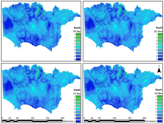
Seasonal groundwater depth (Ds) rating values for (a) spring, (b) summer, (c) autumn, (d) and winter; rating values shown on the right side of the maps.
Net recharge (R)
This study uses recharge values from a transient groundwater model45 using monthly recharge data. The calibrated results for the steady-state and transient model normalized RMS errors were 2.47% and 2.24%, respectively. MODFLOW inputs were provided by Biosym within the Ensym model45. The method used to calculate recharge is described in the Australian groundwater modelling guidelines56. Seasonal recharge values were plotted in ArcMap 10.4.1 and categorized using values from Table 4. The groundwater recharge factor offers significant information to the model, as water recharge is the major driving mechanism for pollution transport57. Additionally, it provides specific information for both spatial and temporal variability. Monthly recharge values for the period from 1987 to 2017 were considered for this analysis. Seasonal recharge maps are shown in Fig. 4.
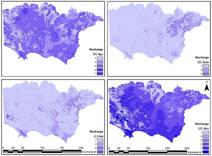
Seasonal net recharge (R) rating values for (a) spring, (b) summer, (c) autumn, and (d) winter; rating values shown on the right side of the maps.
Aquifer media (A)
Aquifer media (A) serves as a conduit for aquifer pollution; the larger the grain size and the more fractures there are in the aquifer, the greater the pollution potential23. The aquifer medium or media are responsible for controlling the route and path length for a contaminant to flow; the larger the porosity of the aquifer is, the lower the attenuation capability, and therefore, the larger the pollution potential. Aquifer configuration materials were obtained from the Victorian Aquifer Framework (VAF)58. The lithological units were categorized with new rating values from 1 to 9 and are presented in Table 5. Next, values were modified from Aller et al.23,43 and adapted to the Victoria geological units (see Fig. 5a).
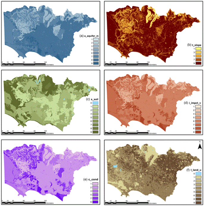
Rating values for (a) aquifer media, (b) topographic slope, (c) soil, (d) impact of vadose zone, (e) hydraulic conductivity, and (f) land use. Rating values shown on the right side of the maps.
Soil media (S)
Soil media is the upper portion of the vadose zone; it has significant biological activity, and it is considered the upper weathered zone of the Earth, averaging six feet (1.8 m) or less23. Soil media control recharge and contaminant attenuation processes such as filtration, biodegradation, sorption, and volatilization23. The upper portion of the soil configuration is used for this factor. Data were extracted from the Atlas of Australian Soil (ASRI), and the variable that represents the topmost layer is (TEXT_TOP) within the Australian Soil Atlas Dataset. The categorization of the Australian soil texture is found in the glossary of soil terms and in “Estimation of Soil Properties using the Atlas of Australian Soils”59. A rating for soil texture groups is presented in Table 6, and the map for the soil media is shown in Fig. 5c.
Topography slope (T)
Topography refers to the slope and slope variability in the land surface; it controls the probability of a contaminant running off or remaining on the surface in a specific area long enough for it to enter the aquifer23. The topography is described in terms of slope percentage41, and the topography slope map was constructed from the digital elevation model (DEM) using ArcMap10.4.1, with a cell size of 50 m × 50 m. The slope was then categorized according to the slope rating values, as shown in Table 7. Figure 5b illustrates the slope % for the study area.
Impact of vadose zone (I)
The vadose zone is defined as the zone above the water table that is unsaturated; it lies below the soil horizon and above the water table30. In the vadose zone, attenuation processes such as biodegradation, neutralization, filtration, chemical reaction, volatilization, and dispersion are likely to decrease as depth increases23. The rating for the vadose zone map was created using the groundwater flow system (GWFS) and the material conformation for each of the aquifer types; conformation material is described in the Victorian aquifer framework49. Table 8 shows the vadose zone ranges and rating values proposed for the Pesticide DRASTICL model. Figure 5d shows the impact of the vadose zone map categorized with the rating values of the modified Pesticide DRASTICL model.
Hydraulic conductivity of the aquifer (C)
Hydraulic conductivity (C) is the aquifer’s material capability to transmit water; it controls the flow rate of groundwater at a given hydraulic gradient, intergranular porosity, tectonic lineaments, and bedding planes23. Similarly, contamination is controlled by the flow rate of groundwater41. Furthermore, C controls the contamination movement in the aquifer23. Within index-based methods, C is denoted as the factor with the highest error associated with its estimation60. The factor rating for C was obtained from two sources. The first is an inferred value from various reports included in the GH GWFS by Dahlhaus et al.48 The second is the data containing conductivity values from a groundwater transient model by SKM45. In this study, k values (m/d) were used from SKM45. A new rating scale is assigned to each range of hydraulic conductivity, as shown in Table 9. A rating map for C is shown in Fig. 5e.
Land use (L)
Changes in land use induce the application of agricultural chemicals, industrial waste spills and landfill leachate, which can potentially leach into groundwater. L is a decisive and inducing factor of aquifer contamination thorough anthropogenic activities60. Research shows that specific methods that integrate information about land use perform better than intrinsic approaches61. Specifically, land use provides additional information on the use of the actual landscape, the type of cropping and crop rotation, which can be used to identify the amount and type of agricultural products used in the catchment61. This approach has been successfully applied in India43, Iraq, Saudi Arabia62,63, Greece64, Portugal25,65, United Kingdom, United States23,66 and Australia67.
Data from 2016 were downloaded from Agriculture Victoria (2018)51, and we selected the secondary land use cell of the Victorian land use information system (VLUIS) to assign new rating values from 1 to 9, as shown in Table 10. Figure 5f shows the land use rating map. Additionally, it shows the land use rating values for different land uses. Next, a raster file was created including the new ratings.
Multivariate statistical assembly of seasonal groundwater vulnerability
In standard DRASTIC methods, GWV has been estimated as a fixed or static value. However, such methods have failed to depict the impacts of temporal variations. Vulnerability can be affected by several factors, such as groundwater extraction, temporal variations in precipitation and evapotranspiration rates, temporal variations in groundwater depths, and temporal variations in groundwater recharge.
To make the vulnerability index sensitive to those changes, the proposed multivariate statistical analysis integrates time variations in depth and recharge while estimating seasonal GWV. This was achieved by estimating a GWV value for each season (spring, summer, autumn and winter). For estimating time-variant values, Eq. (1) was transformed into four different GWV estimations as presented below.
$$ {\text{I}}_{{{\text{DSpr}}}} = \, \left( {{\text{Dr}}_{{{\text{Spr}}}} *{\text{Dw}}_{{{\text{Spr}}}} + {\text{ Rr}}_{{{\text{Spr}}}} *{\text{Rw}}_{{{\text{Spr}}}} } \right) + {\text{ Ar}}*{\text{Aw }} + {\text{ Sr}}*{\text{Sw }} + {\text{ Tr}}*{\text{Tw }} + {\text{ Ir}}*{\text{Iw }} + {\text{ Cr}}*{\text{Cw }} + {\text{ Lr}}*{\text{Lw}} $$
(2)
$$ {\text{I}}_{{{\text{DSum}}}} = \, \left( {{\text{Dr}}_{{{\text{Sum}}}} *{\text{Dw}}_{{{\text{Sum}}}} + {\text{Rr}}_{{{\text{Sum}}}} *{\text{Rw}}_{{{\text{Sum}}}} } \right) + {\text{ Ar}}*{\text{Aw }} + {\text{ Sr}}*{\text{Sw }} + {\text{ Tr}}*{\text{Tw }} + {\text{ Ir}}*{\text{Iw }} + {\text{ Cr}}*{\text{Cw }} + {\text{ Lr}}*{\text{Lw}} $$
(3)
$$ {\text{I}}_{{{\text{Daut}}}} = \, \left( {{\text{Dr}}_{{{\text{Aut}}}} *{\text{Dw}}_{{{\text{Aut}}}} + {\text{ Rr}}_{{{\text{Aut}}}} *{\text{Rw}}_{{{\text{Aut}}}} } \right) \, + {\text{ Ar}}*{\text{Aw }} + {\text{ Sr}}*{\text{Sw }} + {\text{ Tr}}*{\text{Tw }} + {\text{ Ir}}*{\text{Iw }} + {\text{ Cr}}*{\text{Cw }} + {\text{ Lr}}*{\text{Lw}} $$
(4)
$$ {\text{I}}_{{{\text{DWin}}}} = \, \left( {{\text{Dr}}_{{{\text{Win}}}} *{\text{Dw}}_{{{\text{Win}}}} + {\text{ Rr}}_{{{\text{Win}}}} *{\text{Rw}}_{{{\text{Win}}}} } \right) + {\text{ Ar}}*{\text{Aw }} + {\text{ Sr}}*{\text{Sw }} + {\text{ Tr}}*{\text{Tw }} + {\text{ Ir}}*{\text{Iw }} + {\text{ Cr}}*{\text{Cw }} + {\text{ Lr}}*{\text{Lw}} $$
(5)
whereID (Spr, Sum, Aut, Win) = seasonal vulnerability indexDr (Spr, Sum, Aut, Win) = depth ratings per seasonDw (Spr, Sum, Aut, Win) = depth weights per seasonRr (Spr, Sum, Aut, Win) = recharge ratings per seasonRw (Spr, Sum, Aut, Win) = recharge weights per season
After calculating the seasonal vulnerability index Eqs. (2–5), we addressed the estimation of a new set of factors weights with the purpose for eliminating the correlation between factors25. This was achieved by separating DRASTICL factors into two hydrogeological groups: the dynamic group (D and R) and the static group (A. S, T, I, C and L). For both groups, an independent CA was performed, and a new set of upscaled factor weights was obtained for each season. CA deals with the subjectivity bias from using expert opinion for allocating factor weights.
This approach to data treatment (static and dynamic factors) is different from the standard index-based methods, which integrate all factor weightings in one multivariate analysis. CA has been selected because it has been shown to be the most adequate method for transforming the interrelated DRASTIC factors into uncorrelated DRASTICL vectors25.
First, the dynamic factors D, R plus a dummy factor (Q) with a constant value of 5 are resampled in ArcMap 10.4.1 using a fishnet at regular intervals of 5 km. The purpose of the sampling is to extract factor rating values at each point. Next, another point resampling is performed for each of the static factors A, S, T, I, C, and L.
Second, a CA is performed to calculate vector loadings for each group. In the case of the dynamic group, a dummy dataset Q with a mean of 5 in rating value is used to assist in the calculation of the vector loadings as CA can only be performed with more than two factors. CA is also performed for the static hydrogeological group using the A, S, T, I, C and L factors. From both groups, factor loading values are derived from the CA, new vector loadings are obtained and represent the uncorrelated value compared to other factors. Such values are called dynamic vectors (D, R and Q loadings) and static vectors (A, S, T, I, C, and L loadings).
Finally, each vector loading is rescaled to the DRASTICL weighting values (1–5) using the harmonization formula25, as shown in Eq. (6). These new sets of weights are called seasonal vector DRASTICL factor weights.
$$ \begin{gathered} v_{j}^{*} = \frac{{W_{j.max} {\text{x }}v_{j.max} – \left( {W_{j.max} – W_{j.min} } \right) {\text{x }}\left( {v_{j.max} – v_{j} } \right)}}{{v_{j.max} }} \hfill \\ 1 \le j \le p \hfill \\ \end{gathered} $$
(6)
wherewj.max = max factor weight in Pesticide DRASTICwj.min = min factor weight in Pesticide DRASTICvj = factor loadings
The CA was computed using R, an open-access software25. New loading values for vector1 (V1) are calculated as mentioned earlier. The calculated loading values from the CA cannot be compared to the Pesticide DRASTICL weighting values because the loadings are presented on a different scale. From Eq. (6), a new set of re-coordinated weighting values from new vector-DRASTICL factor loadings were calculated. Each factor group was treated as a separate multivariate statistical dataset. Re-coordinated weighting values are known as vector-DRASTICL factor weights25.
Estimating the time-variant Pesticide DRASTICL vulnerability
To improve the outputs of the Pesticide DRASTICL method, factor ratings were reduced to a maximum value of 9, and an independent multivariate CA was applied to both factor groups. After rating categorization, a resample is made using a fishnet of 5 × 5 km to obtain point values from each factor. The fishnet is the base for digital sampling of each of the factors included in the CA. The harmonization of scales method was applied to the resulting CA vector loading values, re-coordinating them from 1 to 5. As a result, seasonal Pesticide DRASTICL weighting values were used to estimate seasonal GWV.
The seasonal estimation of the GWV was quantified by using the corresponding seasonal factor weights. Eight raster layers from DRASTICL factors were used to calculate the seasonal ID. The results were mapped in the study area for each of the seasons.
Different values for vulnerability were expected for each season. The vulnerability values could be similar in places where the levels of depth and water recharge had small or no changes, indicating that the aquifer hydrogeological properties are less sensitive to climatic changes. Conversely, vulnerability values should be higher where depth and recharge showed large seasonal changes in depth and recharge.
Consent to participate
By this means, we the authors give explicit consent to participate in the submission of this scientific paper.
